Tricolor-problem (Tissue)
Description
This case study shows a model of the well-known NP-complete problem of 3-col, by means of tissue like P systems.
Model
The corresponding P-Lingua file is the following:
@model<tissue_psystems>

def main()
{
 /* tissue P system skeleton */
 call tricolor_tissue(n,m);
}

def tricolor_tissue(n,m)
{
  call init_cells();
  call init_multisets(n);
  call init_environment(n,m);
  call init_rules(n,m);
}

def init_cells()
{
  @mu = [[]'1 []'2]'0;
}

def init_rules(n,m)
{
  /* r1,i */ [A{i}]'2 --> [R{i}]'2 [T{i}]'2 : 1<=i<=n;
  /* r2,i */ [T{i}]'2 --> [G{i}]'2 [B{i}]'2 : 1<=i<=n;

  /* r3,i */ [a{i}]'1 <--> [a{i+1}]'0 : 1<=i<=2*n+m+@ceil(@log(m))+10;
  /* r4,i */ [c{i}]'1 <--> [c{i+1}*2]'0 : 1<=i<=2*n;
  /* r5 */ [c{2*n+1}]'1 <--> [D]'2;
  /* r6 */ [c{2*n+1}]'2 <--> [d{1},noD]'0;
  /* r7,i */ [d{i}]'2 <--> [d{i+1}*2]'0 : 1<=i<=@ceil(@log(m));
  /* r8 */ [noD]'2 <--> [e,z{2}]'0;
  /* r9,i */ [z{i}]'2 <--> [z{i+1}]'0 : 2<=i<=m+@ceil(@log(m))+5;
  /* r10,i,j */ [d{@ceil(@log(m))+1},A{i,j}]'2 <--> [P{i,j}]'0 : i<j<=n, 1<=i<n;
  /* r11,i,j */ [P{i,j}]'2 <--> [R{i,j},noP{i,j}]'0 : i<j<=n, 1<=i<n;
  /* r12,i,j */ [noP{i,j}]'2 <--> [B{i,j},G{i,j}]'0 : i<j<=n, 1<=i<n;
  /* r13,i,j */ [R{i},R{i,j}]'2 <--> [R{i},noR{j}]'0 : i<j<=n, 1<=i<n;
  /* r14,i,j */ [B{i},B{i,j}]'2 <--> [B{i},noB{j}]'0 : i<j<=n, 1<=i<n;
  /* r15,i,j */ [G{i},G{i,j}]'2 <--> [G{i},noG{j}]'0 : i<j<=n, 1<=i<n;
  /* r16,j */ [noR{j},R{j}]'2 <--> [bb]'0 : 1<=j<=n;
  /* r17,j */ [noB{j},B{j}]'2 <--> [bb]'0 : 1<=j<=n;
  /* r18,j */ [noG{j},G{j}]'2 <--> [bb]'0 : 1<=j<=n;
  /* r19 */ [e,bb]'2 <--> []'0;
  /* r20 */ [e,z{m+@ceil(@log(m))+6}]'2 <--> [T]'0;
  /* r21 */ [T]'2 <--> []'1;
  /* r22 */ [b,T]'1 <--> [S]'0;
  /* r23 */ [S,yes]'1 <--> []'0;
  /* r24 */ [b,a{2*n+m+@ceil(@log(m))+11}]'1 <--> [N]'0;
  /* r25 */ [N,no]'1 <--> []'0;

}

def init_multisets(n)
{
        @ms(1) = a{1},b,c{1},yes,no;
        @ms(2) = D;
        @ms(2) += A{i} : 1<=i<=n;
        @ms(2) += A{e{i,1},e{i,2}} : 1<=i<=ne;
}


def init_environment(n,m)
{
  @ms(0) = A{i},R{i},G{i},B{i},T{i},noR{i},noG{i},noB{i} : 1<=i<=n;
  @ms(0) += a{i} : 1<=i<=2*n+m+@ceil(@log(m))+11;
  @ms(0) += c{i} : 1<=i<=2*n+1;
  @ms(0) += d{i} : 1<=i<=@ceil(@log(m))+1;
  @ms(0) += z{i} : 2<=i<=m+@ceil(@log(m))+6;
  @ms(0) += A{i,j},P{i,j},noP{i,j},R{i,j},G{i,j},B{i,j} : i<j<=n,1<=i<n;
  @ms(0) += b,D,noD,e,T,S,N,bb;
}
Needed files
A first run
In order to load, parse and simulate this model, we need several files:
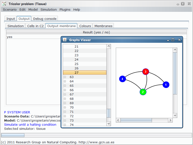
- Custom application, defining the interface with the needed input and output tables for 3-col problem, along with some custom graphs. Install Graphs plugin in order to see the visual representation of the graph and its possible colourations.
- Model file, extracted from :ref:references2 P-Lingua file with the parametrized file specifying the family of P systems for solving the 3-col problem. The custom interface enable the user to introduce the data corresponding to each different scenario.
- Scenario file, for a specific instance of the problem (that is, a specific graph to colour).
Final result
Additional files
Here we provide some additional scenarios:
- Petersen graph.
- Non colorable graph, with 25 nodes including an initial set of nodes making the graph non colorable.
- “Inverse” minimal graph, with 4 nodes, and edges from all the nodes to the last node.
- Minimal graph, with 6 nodes, and edges from the first node to the rest.
- Complete graph, with 8 nodes.
